The Value of ArcGIS Turbo Layers

They’re not for everyone. And you can’t use them all the time. But in the right circumstance turbo layers can put your vector displays on a Starbucks IV.

Actually, the term “Turbo Layer” seems to have fallen out of use (though we kind of like it). Google ArcSDE Turbo Layer and all you get is a reference to a discussion from the year 2000 and other odds and ends. One way to create these is through the use of SDE sdegroup command – though there’s a good bit of discussion about the continuing value of this command. Today we can create these using the ArcToolbox “Dissolve” tool, but we’ll get to that in a bit.

What “turbo layers” are are Geodatabase feature classes created by aggregating the geometries from another class. For example, say you have a class of a 2 million street centerline segments within which there are 100,000 streets – about 20 segments per street. You could create a turbo layer from this class based on street name which would have all lines aggregated to 100,000 multi-part polyline features. Since much of the time required for display involves “fetching” features from the database fetching 100,000 things should be much faster than fetching 2 million things – and in many cases it is.

Also, there’s good article about these in ArcUser Online describing many of the details of this technique, which we won’t go into here. What we will do is to provide a few examples of how they can be used and how you might incorporate them in your enterprise solution.

How Fast is Fast?

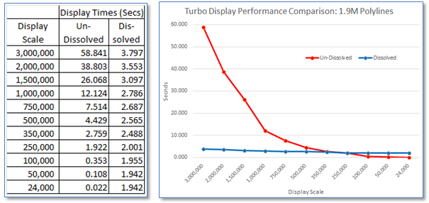
So let’s get down to what kind of performance improvement we’re talking about here. Below we’ve got results of tests performed on a file Geodatabase with a feature class containing approximately 1.9 million polylines and a “turbo layer” class created from it aggregated down to about 130,000 features.  You’re reading that right if you see that at a scale of 1:3,000,000 the full extent of the class, that the original class draws in 58.841 seconds and the turbo layer draws in 3.797 seconds. (Note that all display times listed here were obtained using the ArcGIS PerfQA Analyzer.)

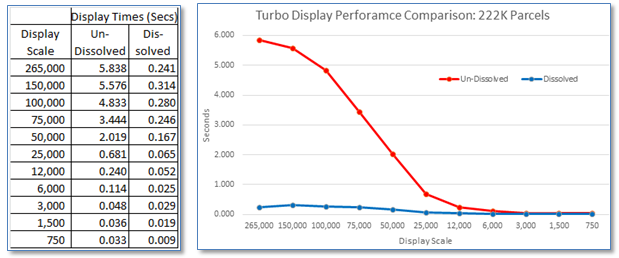
Let’s look at another example. In this case it’s a smaller dataset, approximately 222,000 polylines aggregated down to about 600 based on map number, with a similar pattern to display performance.

What do they look like?

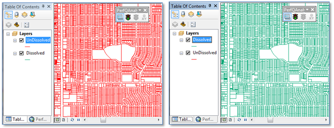
From a pure geographic display point of view, they’re basically identical. As you can see below.  The original, un-dissolved class is on the left in red and the dissolved (turbo) class is on the right in green.

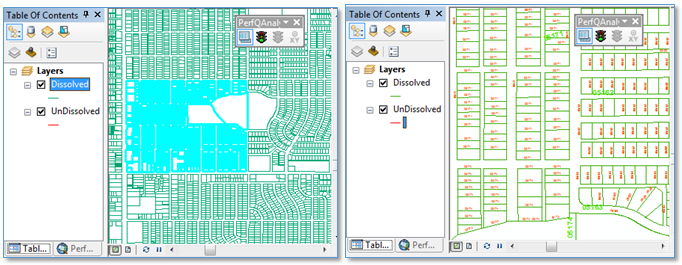
Of course, if you make the turbo layer selectable you’ll get the whole, aggregated feature selected (below left). And if you  want to label the features you’ll get quite different results between the dissolved and un-dissolved versions of the layer (below right).  And if those are requirements, then the turbo layer approach will likely not meet you’re needs.

So What’s the Catch?

Of course there’s a catch. In fact there are several.  It’s up to you decide if the performance gain is worth it.   Here they are:

• Turbo layers are useful for displaying vector geometries of classes with large numbers of lines or points at relatively small scales. The performance difference at relatively large scales is no better and in some cases slightly worse than the original class. The inflection point is reached when the cost of painting the geometry to the display exceeds the cost of fetching data from the database.
• There’s no point in doing an “Identify” or “Select” on the turbo layer – you may as well make it un-selectable. These are for display only.
• They’re useful for static or relatively static data. If the source class does get updated you’ll need a process to re-create the turbo layer either periodically or as-needed.
• Its duplicated data. While there is no point in versioning the turbo layer class – in fact you really don’t want to do this – it will be another feature class in your Geodatabase.
• We’re talking about speeding up vector-based displays.   If you’re generating raster tiles for your Server application, this is probably not for you.
• To use them effectively you’ll need to adjust your current Stored Displays/Map Documents – at least by adding the turbo layer(s) and possibly by setting scale thresholds so that these are shown at small scales and the original data is shown at large scales.

How are Turbo Layers Created?

There are two ways to do this. One is by use of the ArcToolbox Dissolve command found under Data Management | Generalization. This can be automated by 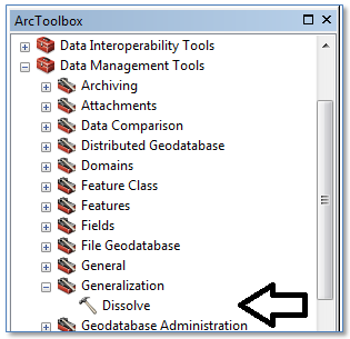inclusion in a python script if you need or want to re-create these regularly.  Dissolve requires a common field on which the features will be aggregated – like a street name, map number, county name, etc.  Finally, while Dissolve retains (by aggregation) all original geometries for lines or points, it eliminates internal boundaries for polygons (thus the name “Dissolve”) – so for polygons you’ll either want to convert these to line features or use option B.

The second way is to use the SDE command line tool SDEGROUP, as mentioned above. SDEGROUP doesn’t rely on a common field for aggregation and takes as a parameter the size of the grid to be used for assembling source geometries into the “grouped” target feature class.  While we know that Esri is in the process of migrating command line SDE tools to ArcToolbox, the future of the SDEGROUP command is not clear as of this writing.

Summary

You may choose simply to suppress display of your large content layers when you get to a scale where their display is either un-necessary or just too annoyingly slow. But if you really want to display this data even at small scales where showing the original layer would just take too long, then consider “turbo layers.”  You may like them.